Why We Trained Our Own Security Finding Classifier

(And Stopped Trusting Frontier Models to Do It)

‍

Our code review agent produces thousands of security findings. Each one needs a labelsqli, xss, authz_missing, non_security_nitpick drawn from a taxonomy of 54 vulnerability classes. Getting that label right isn’t academic. It’s the lynchpin of everything downstream: filtering noisy results, applying customer-specific suppression rules, and feeding our agent’s learning system so it gets smarter about a customer’s codebase over time. A misclassified finding doesn’t just look wrong in a report. It poisons the feedback loop.

We tried three fundamentally different strategies before landing on the one that worked. This post walks through each, what we learned, and why we ultimately fine-tuned a 350-million-parameter open-source model that runs in 21 milliseconds per classification.

The Classification Problem

To understand why this matters, it helps to know how our analysis pipeline is structured. DryRun runs multiple specialized analyzers. Some are what we call “high-signal analyzers,” — focused on well-understood vulnerability classes like SQL injection or XSS. These analyzers already know what they’re looking for. When they flag a finding, the classification is implicit: the analyzer that found it tells you what it is. The patterns are well-defined, and the language and framework signals our agents collect make the classification straightforward.

Then there’s the General Security Analyzer, which reviews pull requests in real time, and our Deep Scan agent, which performs full-repository security analysis. Both are research agents that find vulnerabilities outside the scope of classical, well-categorized issues: missing authorization checks, business logic flaws, insecure defaults, supply chain risks, prompt injection, IDOR, and the long tail of security issues that don’t fit neatly into a pattern-matching box. Both also run high-signal checks for known vulnerability classes, but their real value is in everything else.

This is where classification gets hard and where it matters most. A finding arrives as a title, description, and source filename. Something like:

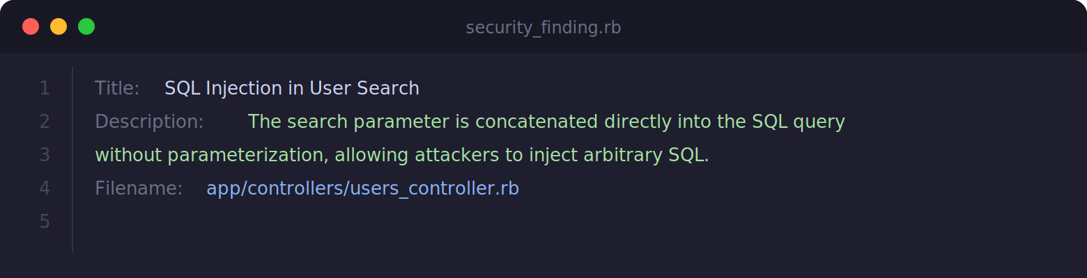
The classifier’s job: map this to one of 54 labels. Some are obvious (sqli). Many are not. Is a missing authorization check authz_missing or idor? Is a weak default configurationinsecure_defaults or anon_security_nitpick? These ambiguities aren’t edge cases. They’re the norm for the General Security Analyzer’s output. Security finding classification sits in a space where categories overlap by nature, and the boundaries between them are genuinely contested even among human reviewers.

Why Classification Accuracy Matters So Much

Classification isn’t a reporting nicety. It sits on the hot path for multiple critical behaviors in our system.

First, it lets us apply category-specific controls to reduce noise. If you know a finding belongs to a particular vulnerability family, you can route it through the right suppression rules, ranking logic, and post-processing behavior. That’s much harder when every finding is just unstructured free text. When a customer tells us “stop flagging informational disclosure findings in our test fixtures,” that rule is only as good as the label. Ifinformation_disclosure findings are being tagged as insecure_defaults, the rule doesn’t fire and the customer sees noise.

Second, classification is one of the inputs to our feedback and learning systems. Over time, we want the agent to adapt to customer repositories, recurring architecture patterns, and organization-specific expectations. That only works if the system can consistently recognize what kind of issue it’s dealing with in the first place. We’ll write more about the learning system in a future post, but the short version is: garbage labels in, garbage behavior out.

Third, classification creates the foundation for meaningful aggregation. Secure code review outputs become much more useful when you can reason in terms of patterns — recurring authorization failures, repeated information disclosure issues, rising supply chain concerns. Without stable labels, none of that analysis is possible.

In other words, if classification is unstable, everything downstream gets noisier.

‍

Attempt 1: Just Ask a Frontier Model

The most obvious approach: send each finding to a large language model along with the full label taxonomy and let it classify. We tested this with frontier-class models including Codex 5.1 Max. The prompt included all 54 label definitions, decision criteria for ambiguous cases, and one example per label.

It worked — sort of. Accuracy ranged from 78% to 85% depending on the run, which is the core of the problem.

Run the same batch of findings twice, and you’d get different labels for a meaningful percentage of them.

The model would waffle on boundary cases: calling something authz_missing on Monday and idor on Tuesday. Temperature 0 helped but didn’t eliminate the variance, especially on the ambiguous cases that matter most.

This non-determinism is a dealbreaker for a system that needs to apply rules and learn from its own output. If the same finding can get two different labels depending on when you ask, your entire downstream pipeline is built on sand.

There were also practical concerns. Every classification required an API call — added latency, added cost, and an external dependency in a critical path. At the volumes we process, those API costs add up fast. And any connectivity hiccup means classifications stall.

Attempt 2: Vector Similarity With RAG

Our next idea: build a reference library. We classified a large set of findings, embedded them into a vector store, and at classification time retrieved the most similar examples. The intuition was sound—if you’ve seen a finding like this before and labeled it the same way, the new one is probably in the same category too.

We tried two variants. Pure vector similarity used nearest-neighbor voting: embed the finding, pull the top-K neighbors from the index, and if enough neighbors agree on a label, use it. We experimented with both local FAISS indices (using OpenAI embeddings) and Pinecone (using AWS Bedrock Titan embeddings) to see if the embedding model or index implementation mattered.

The pure vector approach was fast and less varied, but it struggled with anything novel or ambiguous. It was essentially a lookup table with fuzzy matching, and when the closest examples in the store were themselves borderline cases, the voting just amplified the confusion. It returned other far too often on findings that a human would confidently label.

The RAG variant improved things. Instead of voting, we retrieved similar examples and sent them as context to a frontier model, letting the LLM make the final call with grounded references. This handled novel findings better—the model could reason about the examples rather than just count votes. Accuracy was more consistent than the frontier model approach, landing around 80%, but it still wasn’t where we needed it.

But it still inherited the core problems: API dependency, per-request cost, and inconsistency. The LLM was better-grounded now, but it was still an LLM making judgment calls that could vary between runs. And we’d added the cost and complexity of maintaining a vector store on top of the API calls.

Attempt 3: Fine-Tuning a Small Model

Here’s where things got interesting. We decided to try fine-tuning a small, open-source model specifically for our classification task. The hypothesis: a model that’s seen thousands of labeled examples of exactly this task should outperform a general-purpose model reasoning from descriptions alone, and it should do so without the run-to-run variation we kept hitting.

Choosing the Base Model

Picking a base model wasn’t a single decision — it was a tournament. We started by evaluating several models in the 1B to 9B parameter range on our classification task without any fine-tuning, just prompting with the full label taxonomy. We wanted to see which architectures had the strongest baseline intuition for code and security-related classification.

The Granite family stood out. IBM’s Granite models consistently outperformed comparably-sized alternatives on code-related and security-adjacent tasks in the untrained evaluations — they seemed to have a better innate sense of what security findings are describing, likely owing to IBM’s focus on enterprise and code-heavy training data.

From there, we fine-tuned three candidates head-to-head: IBM’s Granite 4.0 at 350M parameters, Granite at 1B, and Qwen3 at 4B. The expectation was that larger models would win — more parameters, more capacity, better accuracy. That’s not what happened. The 350M Granite model matched or beat both larger models after fine-tuning on our balanced training set.

Our hypothesis for why: the classification task is well-constrained. The input is structured (title, description, filename), the output is a single token from a fixed set of 54 labels, and the decision boundary is defined by the training data. A 350M-parameter model with a hybrid Transformer+Mamba Mixture-of-Experts architecture has more than enough capacity for this task, and the smaller model may actually benefit from having fewer parameters to overfit with.

The practical implications sealed the decision:

• Small enough to serve on a single GPU or an Apple Silicon laptop
• Apache 2.0 licensed — no enterprise licensing headaches
• The hybrid architecture handles long context efficiently, which matters because our system prompt includes all 54 label definitions
• At 350M parameters, it’s roughly 1,000x smaller than the frontier models we’d been calling via API

Building the Training Dataset

The dataset pipeline had three stages.

Stage one: labeling real findings as seeds. We pulled unique security findings from our production database and classified them using a frontier model/human review with the full taxonomy. These labeled real findings weren’t the training data themselves — they were the seed corpus. We needed a large, accurately labeled reference set so we could understand the distribution of vulnerability types in the wild and have high-quality examples to drive synthetic generation.

Stage two: building a balanced synthetic training set. Our real-world distribution has a massive long tail — information_disclosure findings vastly outnumber csv_injection. Training directly on this distribution would produce a model that’s great at common categories and useless at rare ones. So we used the labeled real findings as seeds to generate synthetic training data. For each label, we sampled real examples as context and asked a frontier model to produce realistic variations — findings that read like something our analyzers would actually produce, but with enough variation to teach the model the category rather than memorize specific phrasings. Overrepresented labels were capped; underrepresented labels were synthesized up to a minimum threshold. Every synthetic sample was tagged so we could track its provenance.

Stage three: stratified evaluation split. Critically, our test set is drawn from real findings, not synthetic ones. We held out a stratified portion of the labeled real findings for evaluation, preserving label proportions. Labels with very few real samples were collapsed into other. This means the model is trained on synthetic data but evaluated on production findings — which is the only honest way to measure whether the synthetic training actually generalizes.

Training

We fine-tuned with QLoRA (quantized Low-Rank Adaptation) using the Unsloth library. Rather than updating all 365 million parameters, LoRA trains small adapter matrices — about 13 million parameters, roughly 3.6% of the total model. This keeps training fast and memory-efficient.

The key architectural decision wastrain_on_responses_only. Each training sample is a chat-format conversation: system prompt with all 54 labels, user message with the finding, assistant response with just the label. Without response-only training, ~95% of the gradient signal gets wasted on learning to reproduce the static system prompt. Masking the loss on system and user tokens focuses all learning capacity on the actual classification decision.

Training ran for 3 epochs on an H100, with a learning rate of 2e-4 and effective batch size of 32. Total wall-clock time was measured in minutes, not hours. Final training loss: 0.1164.

After training, we merged the LoRA adapters back into the base weights and exported at 16-bit precision. The result is a self-contained model — no adapter loading, no base model dependency at inference time.

Results

We benchmarked all seven approaches (frontier model prompting, two vector similarity variants, two RAG variants, the fine-tuned model, and a hybrid deterministic+fine-tuned approach) against the same held-out test set.

The fine-tuned Granite model hit 86.6% accuracy across all 54 categories at 21 milliseconds per sample with zero errors across the full test set.

To put those numbers in context:

‍

The accuracy beats the frontier model’s best runs and is stable across every invocation. The speed, cost, and consistency advantages are not close.

Where It Excels

Categories with clear, distinctive patterns scored above 0.95 F1: path traversal, remote code execution, resource exhaustion, excessive privileges, open CORS, XXE. These findings have characteristic language that the model locks onto reliably.

The access control family—idor, authz_missing, excessive_privileges—all scored above 0.88 F1, which is notable because these are genuinely hard to distinguish even for human reviewers.

Where It Struggles

The hardest categories fall into three clusters.

The security-vs-nitpick boundary. non_security_nitpick, insecure_defaults, andbusiness_logic_flaw form a confusion cluster. The model correctly identifies ~73% of non-security nitpicks, but the boundary between “bad practice with no real security impact” and “misconfiguration that could be exploited” is legitimately fuzzy. This is the same boundary human security engineers argue about.

The dependency family. supply_chain_risk, vulnerable_dependency, andlanguage_version overlap significantly. A finding about an outdated package could reasonably be any of these. The model prefers supply_chain_risk (the broader label) when uncertain, which is arguably the safer default.

The catch-all. other scored 0.49 F1 — expected for a category that’s defined as “none of the above.” It’s inherently noisy and mostly functions as a classifier confidence signal: when the model says other, it’s expressing uncertainty.

Misclassification Patterns Tell a Story

The confusion matrix is one of the most revealing artifacts of this entire project — and it looked dramatically different across approaches.

With untrained models and frontier LLM prompting, the confusion matrix was a mess. Errors were scattered broadly across categories with no discernible pattern. The models would confuse rce with information_disclosure, or label a clear sqli as business_logic_flaw — mistakes that don’t reflect any coherent reasoning about the security domain. The confusion wasn’t just frequent, it was unpredictable. You couldn’t look at the error patterns and extract useful signal about where the taxonomy was ambiguous versus where the model was simply lost.

After fine-tuning, the confusion matrix tightened dramatically. The fine-tuned model’s mistakes are almost always reasonable mistakes — the same mistakes a human reviewer might make. It confusesauthz_missing with idor (both are access control issues). It confuses insecure_defaults withnon_security_nitpick (both are about configuration quality). It confuses supply_chain_risk withvulnerable_dependency (both are about dependency problems).

Three distinct confusion clusters emerged:

• The security-vs-nitpick boundary: non_security_nitpick ↔ insecure_defaults ↔ business_logic_flaw. This is the hardest boundary in the entire taxonomy — when does a bad practice cross from “you should fix this” to “this is exploitable”?
• The access control family: authz_missing ↔ idor ↔ excessive_privileges ↔ auth_bypass. All four are fundamentally about “who can access what,” just at different layers of the stack.
• The dependency family: supply_chain_risk ↔ vulnerable_dependency ↔ language_version. These overlap because a vulnerable dependency is a supply chain risk — the distinction is about specificity.

In other words, the model’s error boundary aligns with the genuine ambiguity in the taxonomy itself. This is exactly the kind of confusion matrix you want to see: not random noise, but structured disagreement that mirrors the hard calls human reviewers face.

We’re actively using these patterns to improve. The confusion matrix isn’t a static report card — it’s an engineering input. We’re refining label definitions where the taxonomy creates artificial ambiguity, generating targeted synthetic data for the highest-confusion pairs, and exploring hierarchical classification that groups related labels (the access control family, the dependency family) so the model can get the family right even when the specific label is arguable. Each round of retraining tightens the matrix further. The remaining accuracy gains are likely to come as much from refining the taxonomy — collapsing or clarifying confusing label pairs — as from model improvements.

What We Learned

Consistency matters more than peak accuracy. A model that’s 88% accurate but gives different answers on different runs is less useful than one that’s 86% accurate and stable. Across our benchmarking, the fine-tuned model showed no variation between runs on the same inputs — not because small models are inherently deterministic (they’re not), but because the task is constrained enough and the model confident enough that the outputs didn’t shift. That kind of stability is what downstream systems — rules, learning, reporting — depend on.

Small models can punch above their weight on narrow tasks. 350 million parameters is tiny by modern standards, but when the task is well-defined (54-class text classification from structured input), you don’t need a model that can also write poetry and explain quantum mechanics. Task-specific fine-tuning is a multiplier.

Synthetic data works if you’re careful. Training on LLM-generated data sounds like circular reasoning, but the key is the evaluation boundary. Real labeled findings seed the generation, synthetic data does the training, and real held-out findings do the evaluation. The model never sees the test set during training, and the test set is never synthetic. The synthetic data just fills gaps in the long tail of your label distribution so the model doesn’t ignore rare categories.

The real competition is between approaches, not models. We didn’t spend weeks agonizing over which base model to use. The bigger decision was the strategy: prompting vs. retrieval vs. fine-tuning. Once we committed to fine-tuning, the specific model choice was driven by practical constraints (size, license, architecture, base performance) rather than benchmark chasing.

Invest in your benchmark harness early. We built a reusable framework that let us test any new approach against the same test set with consistent metrics. When you’re comparing seven approaches, having reproducible, apples-to-apples evaluation isn’t a nice-to-have — it’s the only way to make a defensible decision.

What’s Next

The classifier is now a production component, but the real payoff is what it enables. Accurate, consistent labels are the foundation for our agent learning system — the mechanism by which our code review agent improves over time on a customer's specific codebase and security posture. We'll write about that system in an upcoming post.

On the classifier itself, we're already iterating on the confusion clusters described above — tightening label definitions, generating targeted training data for high-confusion pairs, and exploring hierarchical classification. We're also working on confidence calibration using model logits so downstream systems can treat low-confidence classifications differently, and building a continuous retraining pipeline as new finding types emerge from the evolving security landscape.

But classification is just the starting point for what small, domain-specific models can do in security tooling. We're now exploring whether the same principle — fine-tune a tiny model on a narrow, well-defined task — can extend beyond labeling findings to actually finding vulnerabilities themselves.

Early results are promising. We're training extremely small models to validate specific vulnerability classes given dataflow and code context. The first target is remote code execution: given a candidate dataflow path and the surrounding code, can a purpose-built model determine whether the RCE is real? Our initial experiments suggest it can — and that these models outperform untrained frontier models on the same task, which mirrors what we saw with the classifier.

The training approach is fundamentally different from classification. Instead of labeled examples, we're generating training data from agent traces — the reasoning chains our security agents produce as they analyze code. This captures not just the final verdict but the analytical process: how a skilled agent follows data from source to sink, what it checks along the way, and how it distinguishes a true positive from a false alarm. Distilling that reasoning into a small model is a different kind of fine-tuning problem, and we're still early, but the direction feels right.

If this pans out, the implications are significant. Instead of relying on expensive frontier models with inconsistent behaviours for every security judgment in the pipeline, we'd have a constellation of cheap, fast, specialized models — one that classifies, one that validates RCEs, one that confirms authorization flaws — each trained on the specific reasoning patterns that matter for its task. The classifier was our proof of concept that this approach works. Now we're scaling it.